With carefully following along the super lovely Responding to your voice tutorial, I’ve managed to build my own hotword detection classifier. Yay! ! I’ve also managed to run it on the Arduino Nano 33 BLE Sense and via WebAssembly in the Browser and Node.js. Yay II!
But now I am wondering what would be the most correct way for the moving average?
The tutorial seems to have a hint on the moving average topic (see “Poor performance due to unbalanced dataset?”) but at least for me is stays a bit vague. My dataset is balanced with roughly 1500 wav files of 1sec durations for every class (noise, unknown and my-hotword).
Hence could someone please elaborate what would be the best moving average approach and why for the “Hello World” example?
Also a dedicated moving average code example would be terrific, so that one can study and understand it in detail while tweaking paprameters. Maybe extending the one of Classification of existing audio files on desktop with an moving average to detect “Hello World” in wav files of arbitrary durations?
Many thanks!
PS. Also many thanks for the super nice Edge Impulse product! Now finally I can design and create in an easy my own simple classifiers! This is exactly what I have been looking for for ages! Please keep up the good work!
Last related question:
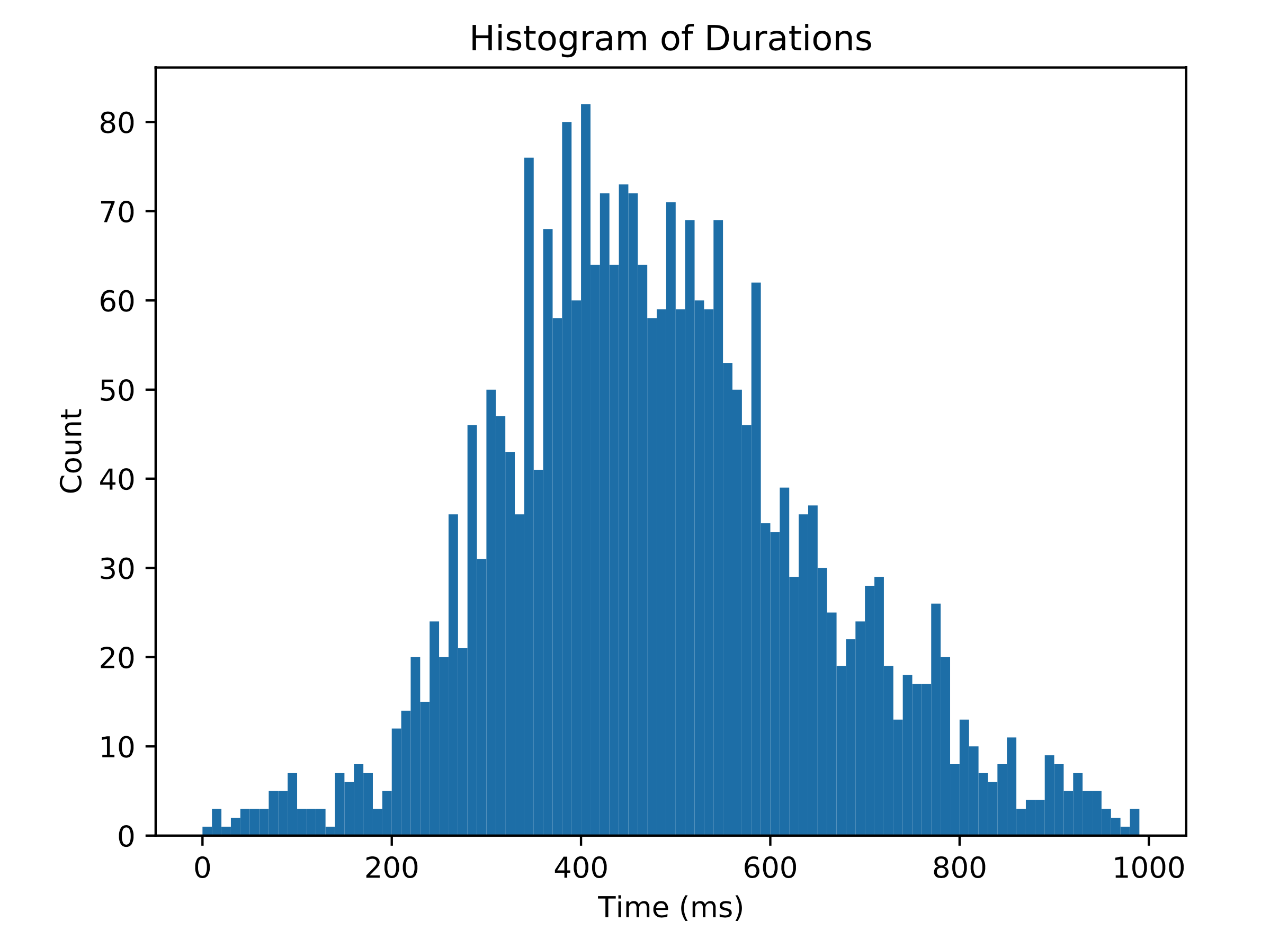
I have a window of 1000ms and currently “centered” all the samples of my hotword inside the 1000ms. The durations of the hotword-sound is divers (see plot below, removed everything under 300 ms in the training data) …
Now I’m wondering why you are exactly slicing into 4 chunks of 250ms. Is this simply due to a compromise of performance on hardware or is there a theoretical reason I don’t get. Would it not be better to classify more often to further increase accuracy?
For others who come across the moving average question, you can see nicely the moving average in action in the “Arduino library” export and the example “nano_ble33_sense_microphone_continuous”:
void loop()
{
bool m = microphone_inference_record();
if (!m) {
ei_printf("ERR: Failed to record audio...\n");
return;
}
signal_t signal;
signal.total_length = EI_CLASSIFIER_SLICE_SIZE;
signal.get_data = µphone_audio_signal_get_data;
ei_impulse_result_t result = {0};
EI_IMPULSE_ERROR r = run_classifier_continuous(&signal, &result, debug_nn);
if (r != EI_IMPULSE_OK) {
ei_printf("ERR: Failed to run classifier (%d)\n", r);
return;
}
if (++print_results >= (EI_CLASSIFIER_SLICES_PER_MODEL_WINDOW)) {
// print the predictions
ei_printf("Predictions ");
ei_printf("(DSP: %d ms., Classification: %d ms., Anomaly: %d ms.)",
result.timing.dsp, result.timing.classification, result.timing.anomaly);
ei_printf(": \n");
for (size_t ix = 0; ix < EI_CLASSIFIER_LABEL_COUNT; ix++) {
ei_printf(" %s: %.5f\n", result.classification[ix].label,
result.classification[ix].value);
}
#if EI_CLASSIFIER_HAS_ANOMALY == 1
ei_printf(" anomaly score: %.3f\n", result.anomaly);
#endif
print_results = 0;
}
}
Hi @b_g it’s a tradeoff about inferences per second and performance. A classification step consists of:
Building a spectrogram of some sorts (MFCC, MFE or normal spectrogram)
Normalizing the data
Running classifier
When we do continuous audio classification we can shorten step 1 significantly (because we only make part of the spectrogram) but 2 & 3 need to run every time we process a slice (on the full spectrogram), so the 4 slices is the balance where we have enough time to do all this on most development boards. If you have a dev board that is faster you can up this freely (see model_metadata.h for the macro). Just look at the DSP+NN timings after each inference, if it’s way less than 250ms. you can safely up this.
 ! I’ve also managed to run it on the Arduino Nano 33 BLE Sense and via WebAssembly in the Browser and Node.js. Yay II!